
How to Calculate Compound Interest in Excel (Step-by-Step Guide)
Easily compute your investment growth using our interactive calculator or learn the exact Excel formulas below.
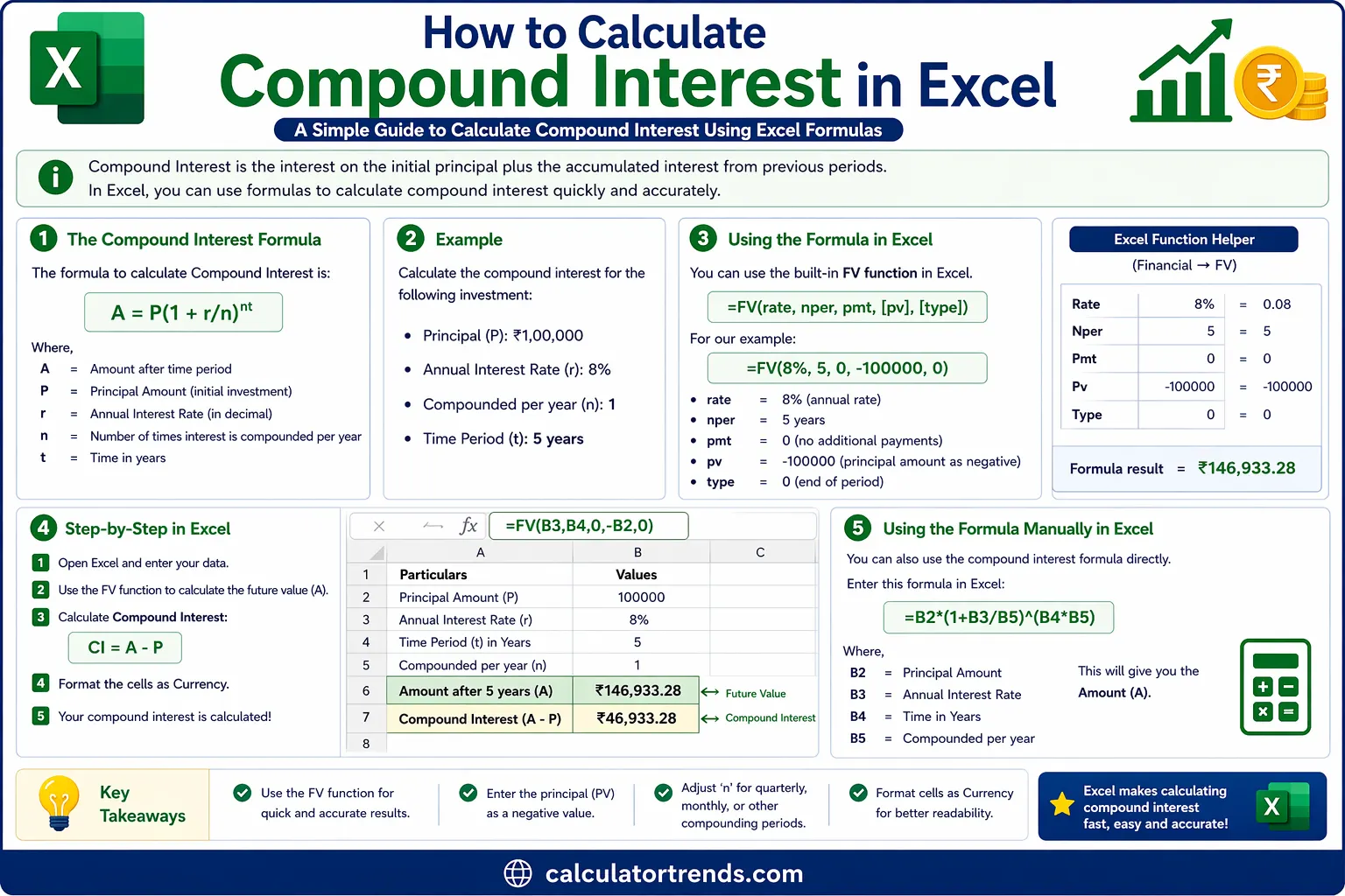
Quick Answer: To calculate compound interest in Excel, use the formula =P*(1+r/n)^(n*t) in any cell, or use the built-in FV function: =FV(rate/n, n*t, 0, -P). Enter your principal, annual rate, compounding frequency, and time — Excel does the rest in seconds.
What is Compound Interest?
Compound interest means you earn interest on your original amount plus the interest already added. Your money grows faster because each period's interest builds on the last.
Say you deposit ₹10,000 at 10% annual interest. After Year 1, you have ₹11,000. In Year 2, interest applies to ₹11,000 — not the original ₹10,000. That extra push is compounding.
Simple interest stays flat. Compound interest snowballs.
Compound Interest Formula
The standard mathematical formula for compound interest is:
| Variable | Meaning | Example |
|---|---|---|
| A | Final amount (principal + interest) | What you're solving for |
| P | Principal — your starting amount | ₹10,000 |
| r | Annual interest rate (decimal) | 10% → 0.10 |
| n | Compounding periods per year | 12 for monthly, 4 for quarterly, 1 for yearly |
| t | Time in years | 5 |
To get only the interest earned, simply subtract the principal from the final amount:
How to Calculate Compound Interest in Excel
There are two reliable methods to perform this calculation in Excel. Both give the exact same answer, so pick whichever feels most comfortable for your workflow.
Method 1: Using the Basic Mathematical Formula
This approach involves typing the math formula directly into a cell, referencing your input variables.
Step 1 — Open a blank Excel sheet and label your inputs like this:
| Row | Cell A (Labels) | Cell B (Values) |
|---|---|---|
| 1 | Principal | 100000 |
| 2 | Annual Rate | 0.08 |
| 3 | Compounding Per Year | 12 |
| 4 | Years | 5 |
Step 2 — Click cell B5 and type this exact formula:
=B1 * (1 + B2/B3) ^ (B3 * B4)
Press Enter. The cell will show ₹1,48,984.57 — that is your final maturity amount after 5 years.
Step 3 — For interest only, click B6 and type:
=B5 - B1
Result: ₹48,984.57 earned purely from the magic of compounding.
What happened inside the formula:
- B2/B3 divides 0.08 by 12 → yielding a monthly rate of 0.00667
- B3*B4 multiplies 12 × 5 → creating 60 total compounding periods
- (1 + 0.00667)^60 raises the growth factor across all periods
- Finally, multiplying by the principal gives you your future value
You can also replace the ^ operator with Excel's POWER function:
=B1 * POWER((1 + B2/B3), B3 * B4)
Method 2: Using the Excel FV Function
Excel has a built-in FV (Future Value) function designed exactly for this. It is cleaner, less prone to typos, and faster to implement.
Syntax: =FV(rate, nper, pmt, [pv], [type])
| Parameter | What to Enter | Our Example |
|---|---|---|
| rate | Interest rate per period (annual rate ÷ n) | 0.08/12 |
| nper | Total number of periods (n × t) | 12*5 |
| pmt | Payment each period (0 if no extra deposits) | 0 |
| pv | Present value — enter as negative | -100000 |
| type | 0 = end of period, 1 = beginning (optional) | 0 |
Step 1 — Using the same input cells as before (B1 through B4).
Step 2 — In cell B5, type:
=FV(B2/B3, B3*B4, 0, -B1)
Press Enter. Result: ₹1,48,984.57
Example Calculation in Excel
Let's walk through a real scenario with actual numbers.
Scenario: You invest ₹2,00,000 in a fixed deposit at 7.5% annual interest, compounded quarterly, for 8 years. How much do you get back?
Set up your sheet:
| Row | A | B |
|---|---|---|
| 1 | Principal | 200000 |
| 2 | Annual Rate | 0.075 |
| 3 | Compounding/Year | 4 |
| 4 | Years | 8 |
Using the basic formula in B5: =B1 * (1 + B2/B3) ^ (B3 * B4)
Using FV in B5: =FV(B2/B3, B3*B4, 0, -B1)
Result: ₹3,62,384.54
Interest earned: ₹3,62,384.54 − ₹2,00,000 = ₹1,62,384.54
Monthly vs Yearly Compounding in Excel
The more frequently interest compounds, the more you earn. Here's the difference on a ₹1,00,000 investment at 10% for 5 years based on the compounding frequency:
| Compounding | n Value | Formula in Excel | Final Amount |
|---|---|---|---|
| Yearly | 1 | =FV(0.10/1, 1*5, 0, -100000) | ₹1,61,051 |
| Quarterly | 4 | =FV(0.10/4, 4*5, 0, -100000) | ₹1,63,862 |
| Monthly | 12 | =FV(0.10/12, 12*5, 0, -100000) | ₹1,64,531 |
| Daily | 365 | =FV(0.10/365, 365*5, 0, -100000) | ₹1,64,866 |
Monthly compounding earns ₹3,480 more than yearly compounding on the same principal and rate. Daily pushes it slightly further. The gap widens dramatically with larger amounts and longer time frames.
Common Mistakes in Excel Calculations
- Entering rate as a whole number: Typing 10 instead of 0.10 for 10% inflates your result absurdly. Always convert: divide by 100 or type the decimal directly.
- Forgetting to divide rate by compounding periods: =FV(0.10, 60, 0, -100000) treats 10% as the monthly rate. You need =FV(0.10/12, 60, 0, -100000). Massive difference.
- Mixing up nper: If compounding monthly for 5 years, nper = 60, not 5. Always multiply: n × t.
- Ignoring cell formatting: A cell formatted as text won't calculate. Right-click → Format Cells → Number or Currency.
Tips to Use Excel for Interest Calculations
- Use named cells. Select B1, click the Name Box (left of formula bar), type Principal. Now your formula reads =FV(Rate/N, N*Years, 0, -Principal) — far easier to audit.
- Build a comparison table. List different rates in column A, different time periods across row 1, and fill the grid with FV formulas. One glance shows your best option.
- Lock cells with dollar signs. When copying formulas across rows, use $B$2 to keep references fixed.
- Try Goal Seek for reverse calculations. Go to Data → What-If Analysis → Goal Seek. Set the final amount cell to your target, and let Excel find the required rate or time.
- Format currency properly. Select your result cells → Ctrl+1 → Currency → choose ₹ symbol and 2 decimal places.
Frequently Asked Questions (FAQs)
What is the compound interest formula in Excel?
How do I calculate monthly compound interest in Excel?
Why does Excel's FV function return a negative number?
Can I calculate simple interest in Excel too?
How do I find what interest rate I need to reach a target amount?
What if I make regular monthly deposits along with my initial investment?
Is there a difference between POWER and ^ in Excel?
Conclusion
The compound interest formula in Excel takes under a minute to set up — whether you type the math directly or use the FV function. Plug in your principal, rate, compounding frequency, and time, and Excel handles the rest. Start with the FV method if you want fewer errors and cleaner sheets, and save your file as a reusable template so every future calculation takes seconds instead of starting from scratch.